Reinforcement Learning for drone networks
Implementation of both routing algorithm and MAC protocol for networks of drones using reinforcement learning.
Reinforcement Learning-based MAC protocol
Consider the case of a network of drones trying to communicate with a depot, whose purpose is to allocate bandwidth for them to send data.
Reinforcement Learning setting
In this scenario, the depot will represent the agent while the drones with their information define the environment. Due to the lack of information about the drones accessible by the depot, a stateless (i.e., bandit-like) formulation is used as a baseline.
Reward function
The reward function is a value function determining the `goodness’ of a decision (action) and implicitly defines the goal of the problem. In this case, a smooth reward function is considered as the RL process converges faster on this kind of function rather than sparse ones.
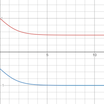
The key idea is that the reward should have high value when the depot chose a drone which has packets to upload and the expired packets are few (possibly 0), while it should have low value (negative in our case) if the depot queries a drone that has no packet to deliver; the more the expired packets, the lower the value of the reward. For additional regularizing effect, the reward is restricted to be in the range \([-1;1]\). Let \(D_t\) be 1 if the drone queried at time \(t-1\) had a packet to deliver, and \(F_t\) the feedback returned from the query. Then,
\[\begin{equation*} R(t) = \begin{cases} 1.5 -\frac{1}{1 + e^{-F_t}} & \textit{if } D_t=1 \\ -\frac{1}{1 + e^{-F_t}} & \textit{otherwise} \end{cases} \end{equation*}\]The following shows the trend of the defined reward
Policies
Two different policies are considered in this work:
- \(\varepsilon\)-greedy policy, where the greedy action (drone) is selected with probability \(1-\varepsilon\) and a random action with probability \(\varepsilon\); in this way, we try to define a reasonable trade-off between exploration and exploitation, which is typically a challenge in Reinforcement Learning; Let \(Q_t(a)\) the estimated value of the action \(a\) at time step \(t\), then
- Upper-Confidence Bound} (UCB), which considers how close the estimate of action is to be maximal and the uncertainty in its estimate:
where \(N_t(a)\) denotes the number of times that action \(a\) has been selected before time \(t\), and \(c > 0\) controls the degree of exploration.
The idea of UCB is that the square root term is a measure of the uncertainty in the estimate of \(a\)’s value. Each time \(a\) is selected the uncertainty is presumably reduced since \(N_t(a)\) increments. On the other hand, each time an action other than \(a\) is selected, \(t\) increases but \(N_t(a)\) does not, so the uncertainty estimate increases instead.
Learning models
In order to face this task, two different RL approaches are considered: due to the bandit-like nature of the problem, k-armed bandit represents the baseline; an improvement is achieved using Gradient Bandit.
Finally, the final model is based on Deep Reinforcement Learning, using, in particular, the Double Q-Learning algorithm, which produced the best results altogether.
Gradient Bandit Algorithm
In this setting, the k arms are exactly the drones that the depot can query. The Gradient Bandit algorithm computes preferences of actions \(H\): the larger the preference, the more often the action is taken. Actions are selected accordingly to a softmax distribution \(\pi\) over the preferences. Let \(A_t\) be the action selected at time \(t\) and \(a\) all the actions \(\neq A_t\). \(H\) is then updated in each iteration as:
\[\begin{align*} H_{t+1} (A_t) &= H_t(A_t) + \alpha \left(R_t - \bar{R}_t \right) \left( 1 - \pi_t(A_t) \right) \\ H_{t+1} (a) &= H_t(a) + \alpha \left(R_t - \bar{R}_t \right)\pi_t(a) \quad \end{align*}\]where \(\alpha\) is a step-size parameter and \(\bar{R}_t\) is the average of the rewards.
Observe that using softmax over the \(H\) values of actions also induces a policy given by the discrete distribution of the softmax values.
Double Deep Q-Network
The idea, introduced by Mnih et al., 2015, is that deep neural networks being universal function approximators implies they can also approximate Q-functions.
However, this category of algorithms relies on a stateful representation: that is, the Q-values of actions are conditioned over the state of the environment in which they are evaluated. So, the environment state at time \(t\) is represented as:
- A one-hot vector identifying the drone queried at \(t-1\)
- The miss ratio for each drone (# queried \(a\) and no packet / # queried \(a\))
- The hit ratio for each drone (# queried \(a\) and packet / # queried \(a\))
- The guess ratio for each drone (# queried / \(t\))
For training, the Double DQN algorithm is employed. The idea consists in having two identical networks (one for prediction and the other for evaluation) and only updating the former (the ‘current’ one), while the latter (the ‘target’) has its weights set equal to the former for each \(\tau\) step.
Up to now, DQN training algorithms generally only differ in the chosen loss function:
\[\begin{align*} & L((s,a,r,s'),\mathbf{\theta},\mathbf{\theta'}) = \\ & (r + \gamma Q(s',\underset{a'}{\operatorname{argmax}} Q(s',a',\mathbf{\theta}),\mathbf{\theta'}) - Q(s,a,\mathbf{\theta}))^2 \end{align*}\]where \(\theta, \theta'\) are the weights of the current and target network, respectively, and \((s,a,r,s')\) represents an experience in which the agent applies \(a\) in \(s\), bringing the environment in state \(s'\), and gets reward \(r\).
\(\gamma \in [0,1]\) is a discount factor.
In this formulation, it can be seen that the target network evaluates the greedy action computed by the current network, and this term is compared to the Q-prediction of the action that the agent actually took during exploration.
We also tested the usage of replay buffers, i.e., storing experiences in a buffer and sampling them to train the network in batches, but it yielded worse results than just using the most recent experience (probably due to the length of the training, much shorter than the usual reinforcement learning process, which can easily take days).
Results
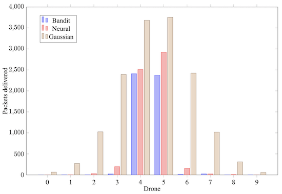
Overall, the best results are given by the double DQN, using UCB as policy. \(\varepsilon\)-greedy would yield results slightly higher in metric but would fail to generalize well (e.g. in the gaussian test case, it would just pick the two majority classes and ignore all the others, while UCB would try to approximate the actual distribution).
Reinforcement Learning-based Routing protocol
In a patrolling scenario where a drone explores an area, a typical issue is sending packets to the depot only after completing the whole path. This behavior may be undesired since it could be important to receive packets quickly to avoid expiration. This homework aims to tackle this issue by implementing a routing protocol that, leveraging a squad of drones, improves the delivery of packets to the depot. We present two different Q-learning-based approaches: the Q-Table model and Double Deep Q-Network.
Reinforcement Learning setting
In this setting, the environment is composed of a squad of \(N\) drones and a depot, with a single drone patrolling the area and the others performing various tasks, and they can be exploited to offload packets and reduce data latency at the depot; in particular, drone 0 can choose to send, or not, a packet to a close-by drone which is responsible of delivering it to the depot when it can. If drone 0 decides to keep a packet, then it will be delivered after completing his route.
So, the agent is drone 0 while the environment is represented by the remaining ones and the depot.
Reward function
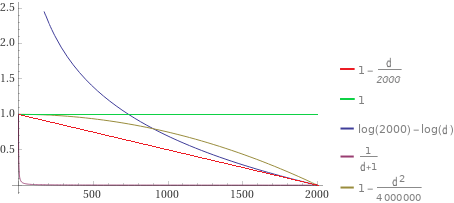
Considering that every time the depot receives a packet, feedback is given to drone 0, and we leverage this feedback to get a value that tells us if the chosen action was good or not. Specifically, the feedback tells us if the packet is delivered correctly or not (respectively \(1\) and \(-1\)), from which drone is delivered and the delay; we use only the first and last information to compute the reward. Let \(d\) be the delay, \(o\) the outcome and \(e\) the delay after which the packet expires (in this case \(e = 2000\)).
The following functions, except the constant one, are monotonic decreasing functions since we want that higher delay leads to lower reward:
-
Logarithmic reward function:
\[\begin{equation*} R(t) = \begin{cases} -log(\frac{d}{e}) & \textit{if } o > 0 \\ -10 & \textit{otherwise} \end{cases} \end{equation*}\] -
Hyperbolic reward function:
\[\begin{equation*} R(t) = \begin{cases} \frac{1}{d+1} & \textit{if } o > 0 \\ -1 & \textit{otherwise} \end{cases} \end{equation*}\] -
Linear reward function:
\[\begin{equation*} R(t) = \begin{cases} -\frac{d}{e}+1 & \textit{if} o > 0 \\ -1 & \textit{otherwise} \end{cases} \end{equation*}\] -
Quadratic reward function:
\[\begin{equation*} R(t) = \begin{cases} -(\frac{d}{e})^2+1 & \textit{if } o > 0 \\ -1 & \textit{otherwise} \end{cases} \end{equation*}\] -
Constant reward function:
\[\begin{equation*} R(t) = \begin{cases} 1 & \textit{if } o > 0 \\ -1 & \textit{otherwise} \end{cases} \end{equation*}\]
Policy
A typical challenge in RL is to define a trade-off between exploration and exploitation to make the model able to look for new good solutions and not only exploit greedy ones.
The \(\varepsilon\)-greedy policy is the easiest way to implement this trade-off; in particular, with probability \((1 - \varepsilon)\) it returns the greedy action, while with probability \(\varepsilon\) it returns a random action, namely the model explores the action space:
\[\begin{equation*} A_t = \begin{cases} \displaystyle{\underset{a}{\operatorname{argmax}}} \ Q_t(a) &\mbox{wp } 1-\varepsilon \\ \textit{a uniformly random action} &\mbox{wp } \varepsilon \end{cases} \end{equation*}\]Learning models
The two approaches implemented to solve the task are:
- Q-Table model;
- Double Deep Q-Learning.
Q-Table model
We define the state space as follows:
\[\begin{equation*} S = H \times I \end{equation*}\]where:
- \(h \in H\) is the number of hops to the depot from the last reached target;
- \(i \in I\) be the index of the cell where drone 0 is located.
We define the action space as follows:
\[\begin{equation*} A =\{d | d \textit{ is a drone}\} \end{equation*}\]Taking action \(d\), drone 0 will use drone d as relay if \(d\) is another drone and keep the packet if \(d\) is itself.
We also need to define the successor \(s'\) of a state \(s\) given a certain action \(a\).
\[\begin{equation*} s' = (h', i') \end{equation*}\]Let \(t\) be the next target which the drone has to reach when it takes the action $a$ in state \(s\), then:
- \(h'\) is the number of hops from \(t\) to the depot;
- \(i'\) is the cell index of \(t\).
To train the model the classic Q-Table algorithm is used, using the following update rule:
\[\begin{equation*} \scriptstyle Q(s,a) \leftarrow Q(s,a) + \alpha\left[R + \gamma \displaystyle{\underset{a' \in A}{\operatorname{argmax}}} Q(s', a') - Q(s, a) \right] \end{equation*}\]Double Deep Q-Network
In this case, the environment state at time \(t\) is represented as follows:
- Coordinates of each neighbor drone (\((0,0)\) for non-neighboring drones);
- Distance of each neighbor drone from the depot;
- Coordinates and distance from the depot of drone \(0\);
- Current step in the route of drone \(0\) (as a one-hot vector).
For training, the Double DQN algorithm is used. Now, the loss is computed as:
\[\begin{align*} & L((s,a,r,s'),\mathbf{\theta},\mathbf{\theta'}) = \\ & (r + \gamma Q(s',\displaystyle{\underset{a'}{\operatorname{argmax}}} Q(s',a',\mathbf{\theta}),\mathbf{\theta'}) - Q(s,a,\mathbf{\theta}))^2 \end{align*}\]Where $\theta, \theta’$ are the weights of the current and target network, respectively, and \((s,a,r,s')\) represents an experience in which the agent applies \(a\) in \(s\), bringing the environment in state \(s'\), and gets reward \(r\).
\(\gamma \in [0,1]\) is a discount factor.
In this formulation, it can be seen that the target network evaluates the greedy action computed by the current network, and this term is compared to the Q-prediction of the action that the agent actually took during exploration.
Furthermore, we used a replay buffer to achieve a regularizing effect. The idea is to store past experiences in a buffer and sample \(N\) to train the network in batches. Ideally, this should allow the model not to `forget’ past experiences. This technique produced an observable performance increase.
Results
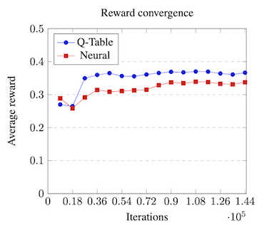
Despite Deep RL giving impressive results in recent works, this setting is probably not the best for such models; in particular, the Q-Table model would consistently outperform the DQN, also achieving faster convergence time. The main motivation behind this result is the number of updates. In particular, the models receive an update for each delivered or expired packet. This number is a lot smaller than the length of the simulation (we get ~30 updates for 18k steps of simulation) and simply not enough to train a neural network well. For this reason, the size of the network has to be limited (the final model has ~800k weights), as a bigger network would achieve better results but would require even more time to converge. This trade-off between expressive power and convergence time led to non-optimal results.
