Natural Language Processing Homeworks
Design and implementation of architectures to face both Named Entity Recognition (NER) task and Semantic Role Labeling (SRL) task.
Named Entity Recognition
The task consisting of classifying every word of a sentence in categories such as a person, organization, location, and others, is called Named Entity Recognition (NER). There are different ways to deal with this kind of task, like unsupervised learning and supervised learning approaches, and the one I chose is supervised learning. With this approach, the NER task can be considered as a sequence labeling task. Initially, with this kind of approach were used hand-engineered features or specialized knowledge resources like gazetteers, but leveraging deep learning techniques to discover features automatically, improved the models until they reached the state-of-the-art.
Recurrent neural networks (RNNs) work very well in modeling sequential data. In particular, bidirectional RNNs can create a context using past information retrieved from the forward states and future information retrieved from backward states for every step in the input. Thus, each token of a sentence will have information about the whole sentence. But it has been proven that in practice, RNNs tend to be biased from the most recent inputs. To avoid this behavior can be used long short-term memory networks which can capture long-range dependencies. Moreover, since in the NER task, to predict the label of each word needs to make use of neighbor tag information, to decode it is used conditional random field.
Neural architecture
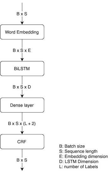
The chosen neural architecture is composed of an embedding layer, followed by a bidirectional long short-term memory with a sequential conditional random layer.
Embedding layer
The input of the model is a vector that represents each word of the given sentence. The representation of every word is done by using an embedding layer that returns a fixed dimensionality real-vector that stores the semantic and syntactic information of words.
Starting with randomly initialized embedding, I observed significant improvements with pre-trained ones. In particular, with pre-trained word embeddings, the model converges very quickly, allowing to get relevant results in fewer epochs as compared with the model which had the randomly initialized embeddings. I tried both Glove J. Pennington et al. 2014, trained using Wikipedia 2014 and Gigaword 5, and fast text E. Grave et al. 2018, trained on Common Crawl and Wikipedia, embeddings to observe that with the latter, I get better performance.
Bidirectional LSTM
Long short-term memories (LSTM) are a variant of the RNNs that use memory cells to propagate information through the sequence without applying non-linearities J. Eisenstein et al. 2019.
The reason for using the bidirectional LSTM is to create the context of each word in the sentence. To do this is used two different LSTM with different parameters. Indeed, the network takes as input a sentence represented as a sequence of \(n\) words, \((x_1, x_2, \dots, x_n)\); each \(x_i\) of the sequence represents a word embedding of the \(i\)-th word of the input sentence. This sequence is fed to a first LSTM, which computes the left context of each token in the sentence, and then another LSTM reads the same sequence in a reverse way to create the right context of the tokens. These two representations are then concatenated to obtain the actual representation of the word in the context. This pair of LSTM is known as Bidirectional LSTM.
Conditional Random Field
Conditional random field (CRF) is a conditional probabilistic model for sequence labelling used when there are dependencies across output labels, like in NER task, since the grammar imposes constraints on the interpretable sequences of labels which are to be modelled jointly, and it is based on the score function:
\[\begin{equation*} \Psi\left( \vec{w}, \vec{y} \right) = \sum_{m = 1}^{M+1} \psi\left(\vec{w}, y_m, y_{m-1}, m \right) \ . \end{equation*}\]To estimate the parameters is needed to maximize the following probability of a label given the word, which is based on the label of the previous word and the current word:
\[\begin{equation*} p(\vec{y} \ | \ \vec{w}) = \frac{e^{\Psi\left( \vec{w}, \vec{y} \right)}}{\sum_{\vec{y'} \in \mathcal{Y}(\vec{w})} e^{\Psi\left( \vec{w}, \vec{y'} \right)}} \ . \end{equation*}\]While to decode the best sequence of labels \(\hat{y}\) which maximizes the previous probability, it is computed efficiently using the Viterbi algorithm, which leverages the dynamic programming technique for reusing work in recurrent computations.
\[\begin{equation*} \hat{y} = \underset{\vec{y}}{\operatorname{argmax}}\Psi\left( \vec{y}, \vec{w} \right) \end{equation*}\]I implement the CRF layer taking inspiration from the following vectorized implementation.
Experiment
This section presents the model setup for the training phase and the outcomes and the workflow of the latter.
Training process
With the purpose of making the sentences readable by the neural network, each sentence is converted into a tensor of numbers, each of which identifies a word in a vocabulary built from the training dataset. Each sentence is then padded to make its length homogeneous; this is useful to work with batches of sentences. These latter are input to the embedding layer, which is initialized using fast text pre-trained embeddings that cover 90% of the vocabulary, and the remaining embeddings are initialized randomly.
The resulting of the embedding layer passed through a dropout layer, with \(p = 0.5\), which drops out some units to prevent overfitting and co-adaptations on training data. Then, tensors outputted by the previous layer are fed to the BiLSTM composed of one layer whose dimension is set to 128.
Thereafter, the output of the LSTM is passed through another dropout layer and a dense layer which outputs the representation of the emission score to give in input to the CRF layer, together with the transition matrix obtained by adding two new labels needed to represent the start and the end of the sentences, which returns the predictions.
Adam optimizer is used with a gradient clipping set to 2.0 (usually used to avoid exploding gradients in RNN). To prevent overfitting, besides the dropout layer, some hyperparameter tuning is done. In particular, the model works fine with a learning rate set to 1e-2 and weight-decay set to 1e-7. The latter is also used to penalize big weights and so penalize the complexity of the model.
With the aim of evaluating the model, the negative log-likelihood is used as a loss function instead of likelihood because computing the partial derivatives of the logarithm are easier than the partial derivatives of the softmax equation, and it must be minimized since minimizing the negative will yield the maximum.
Results
The metrics used to evaluate the model are the macro precision, macro f1, and macro recall that are computed independently for each class. The model is trained for 10 epochs where each epoch takes approximately 2 minutes, reaching about 88% of macro f1 on the test dataset.
As can be seen in the following confusion matrix, most of the wrong predictions are for minority classes, i.e. the labels ‘ORG’ and ‘LOC’; this is the reason for using macro metrics since they consider classes imbalance issues.
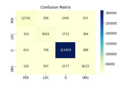
The performances obtained on the dev dataset are
| precision | recall | f1-score | support | |
|---|---|---|---|---|
| PER | 0.92 | 0.89 | 0.90 | 14396 |
| LOC | 0.86 | 0.80 | 0.83 | 12359 |
| O | 0.99 | 0.99 | 0.99 | 315809 |
| ORG | 0.82 | 0.73 | 0.77 | 9043 |
| accuracy | 0.97 | 351607 | ||
| macro avg | 0.90 | 0.85 | 0.87 | 351607 |
| weighted avg | 0.97 | 0.97 | 0.97 | 351607 |
Conclusion
The resulting model is left very simple, making it as generalized as possible so that it does not depend on the task, and still, it can achieve almost the performance of the state-of-the-art models.
Semantic Role Labeling
A fundamental task in Natural Language Processing is the task of Semantic Role Labeling which extracts the predicate-argument structure of a sentence, determining “who did what to whom”, “when”, “where”, and “how”. The whole SRL process is divided into four steps:
- predicate identification: which consists in identifying the predicates in a sentence;
- predicate disambiguation: which consists in determining the type of the identified predicates;
- argument identification: which consists in identifying the arguments in a sentence of a specific predicate;
- argument classification: which consists in determining the role of the arguments in relation to a specific predicate.
For the purpose of the homework, the mandatory tasks are argument identification and argument classification, while the other two are optional.
In this work, two models are presented: one which deals with the tasks argument identification and argument classification, and the other which deals with the tasks predicate disambiguation, argument identification, and argument classification; from now on, in the report, these two models will be respectively named \(M_1\) and \(M_2\).
Since both the tasks argument classification and predicate disambiguation can be seen as sequence labeling tasks, the neural model with which to face these tasks is the bidirectional LSTM that can capture syntactic information leveraging the context created by its states.
Moreover, the two models use a pre-trained BERT model to get the embedding representation of each word of a sentence during the preprocessing of the dataset.
In the next sections are described the structures of the models, the encoding of the input both in \(M_1\) and \(M_2\) with their training and validation phases, and analysis of the experimental outcomes obtained by increasingly improving the models.
Neural architecture
The architectures of \(M_1\) and \(M_2\) are very similar, in particular, \(M_2\) includes \(M_1\) to face the tasks of argument identification and argument classification, but encodes the sentences in a different way.
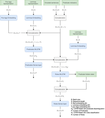
\(M_2\) is composed of two stacked bidirectional LSTM (Long Short-Term Memory), the former LSTM dealing with predicate disambiguation task, while the latter LSTM, leveraging the results of the first, faces the argument identification and classifications tasks. Instead, \(M_1\) is composed of only a bidirectional LSTM that faces the tasks of argument identification and argument classification. Both the models use a pre-trained Bert model during the preprocessing of the dataset to get the embedding representation of the sentence while to represents the other syntactic information D. Marcheggiani et al. 2017 use different embedding layers.
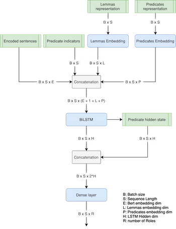
The flow of the developed models are
BERT model
Taking inspiration from P. Shi et al. 2019, during the preprocessing of the dataset, instead of using a pre-trained word embedding, a pre-trained BERT model is used to get the embedding representation of a sentence, which has shown impressive gains in many natural language tasks among which there are the sequence labeling tasks. BERT, which stands for Bidirectional Encoder Representations from Transformers, is a neural model that makes use of Transformer, an attention mechanism that learns contextual relations between words and/or sub-words in a text.
There are many pre-trained models that differ in the number of parameters, and for this work, I adopted the simplest pre-trained BERT model (‘Bert-base-cased’), which has 12 layers, a hidden size equals 768, and the number of self-attention heads equals to 12, for a total number of parameters equals to 110M (as mentioned in J. Devlin et al. 2018);
Embedding layers
With the aim of giving the model more information as possible, the dataset provides much syntactic information. From the set of information, those used are pos tags, predicate frames, and lemmas D. Marcheggiani et al. 2017; these are exploited in different ways in the two models \(M_1\) and \(M_2\), but the thing that has in common is that they are represented using an embedding layer.
After getting the contextual embedding representation of the sentence using the BERT model, depending on the model, the sentence is concatenated the information obtained from the embedding layers.
- \(M_1\): In the following model the sentence is simply represented by the concatenation of all the selected information; so, let \(x_i = x_i^{\text{bert}} \circ x_i^{\text{pred_ind}} \circ x_i^{\text{pos}} \circ x_i^{\text{preds}} \circ x_i^{\text{lemmas}}\) be the representation of the token \(i\) of the sentence where \(\circ\) is the concatenation operator; then, \(x_i^{\text{bert}}\) represents the contextual embedding of the token \(i\), \(x_i^{\text{pred_ind}}\) represents the predicate indicator of the token \(i\) which is 1 if \(x_i\) is a predicate 0 otherwise, \(x_i^{\text{pos}}\) represents the embedding of the pos tag of the token \(i\), \(x_i^{\text{preds}}\) represents the embedding of the predicate frame of the token \(i\) and \(x_i^{\text{lemmas}}\) represents the lemma embedding of the token \(i\);
- \(M_2\): since this model is composed of two bidirectional LSTM where the latter leverages the output of the former, a different representation is adopted. To the first LSTM that faces predicate disambiguation task, the sentence is fed to it with only the information useful to disambiguate the predicates, so \(x_i^{\text{LSTM}} = x_i^{\text{bert}} \circ x_i^{\text{pred_ind}} \circ x_i^{\text{pos}} \circ x_i^{\text{lemmas}}\), but to add more relevance to the token that represents the predicate, \(x_i^{\text{lemmas}}\) is the embedding of the lemma of the token \(i\) only if in position \(i\) there is a predicate, while about the pos tag embedding is better to have information about all the tokens because to disambiguate a predicate is useful also know what part of speech the other tokens play in the sentence. The second LSTM that composes \(M_2\) leverages the output of the previous LSTM to face the tasks of argument identification and argument classification. So, the representation of each token of a sentence is the following \(x_i = x_i^{\text{bert}} \circ x_i^{\text{LSTM}} \circ x_i^{\text{lemmas}}\) where in this case the embeddings of the lemmas are all used. Note that the pos tag embeddings are not used since in \(x_i^{\text{LSTM}}\) there is already the information about them.
BiLSTM
Long short-term memories (LSTM) are a variant of the Recurrent Neural Networks that use memory cells to propagate information through the sequence without applying non-linearities. The reason for using the bidirectional LSTM is to create the context of each word in the sentence using two different LSTM: one which computes the left context of each token in a sentence and a second LSTM which reads the same sequence in a reverse way to create the right context of the tokens; the two contexts are concatenated to obtain the representation of each token in the sentence.
In both the models \(M_1\) and \(M_2\), before doing role classification, the hidden state of the predicate returned by the LSTM is concatenated to the hidden state of each token of the sentence and then fed into a fully connected layer to do the classification; this is done to add more dependency from the predicate to each token of the sentence P. Shi et al. 2019.
Experiment
The models are built increasingly starting from using only the word embedding to represent the sentence until using almost all the syntactic information given in the dataset.
Encoding of the input
To represent the sentences, some vocabularies are made to represent all the information about the pos tags, the lemmas, the predicates, and the roles (this is necessary to evaluate the performances of the model). After verifying that all the pos tags and roles that are in the validation and the test dataset are also in the training dataset, their vocabularies are built using only the information in the provided dataset; while, about the vocabulary of the predicate frames, I used VerbAtlas (A. Di Fabio) which provides all the possible frames avoiding the use of ‘\(\langle\)unk\(\rangle\)’ token, which is instead necessary to build the vocabulary of the lemmas.
Due to the fact that in the dataset there are sentences without predicates, these are handled as information of relevance, but since in the dataset the dictionary of the roles for these sentences is empty, it is replaced with an array filled with the null token; in this way, no information is lost. However, rather it helps the model to identify in a better way which token will be predicted as a null token.
In both the models, the BiLSTM, which predicts the roles, takes as input a sentence with only one predicate in order to predict only the roles that each token of a sentence assume considering that specific predicate and to avoid missing predictions since there can be a token that has a different role for two distinct predicates. So, for the sentences with many predicates, the model, during its forward step, splits them and assigns a predicate to each of these duplicated sentences.
Training phase
The models are trained using Adam optimizer, where the model \(M_1\) has the following hyperparameters
| Hyperparameters | |
|---|---|
| Bert embedding | 768 |
| Pos tags embedding dim | 128 |
| Lemmas embedding dim | 200 |
| Predicate embedding dim | 200 |
| Hidden dim | 512 |
| Batch size | 128 |
| Dropout | 0.2 |
| Learning rate | 1e-3 |
| Gradient clipping | 2 |
while the ones for the model \(M_2\)
| Hyperparameters | |
|---|---|
| Bert embedding | 768 |
| Pos tags embedding dim | 128 |
| Lemmas embedding dim | 200 |
| Predicate hidden dim | 400 |
| Roles hidden dim | 512 |
| Batch size | 128 |
| Dropout | 0.2 |
| Learning rate | 1e-3 |
| Gradient clipping | 2 |
Furthermore, different loss functions are used for the models: since \(M_2\) must face two different tasks, a linear combination of two different losses is used, one cross-entropy function for the task of predicate disambiguation and another cross-entropy function for the task of role classification. About this linear combination, I decided to give more relevance to the loss of the role classification task since it is the main task of the SRL pipeline and also because it is more difficult due to the fact that for predicate disambiguation, the position of each predicate is already known, while for the role classification task is not the same, so the loss for predicate disambiguation task has a weight of 0.4 and the loss for role classification task has a weight of 0.6. While about \(M_1\), only a cross-entropy function is used for the role classification.
To improve the models’ generalization ability and to avoid overfitting, some regularizers are introduced. One of them is the dropout layer which is applied on the whole word representation, on the input, and on the output of the BiLSTM that takes care of the role classification task; moreover, it is even applied to the output of the BiLSTM that takes care about predicate disambiguation task. Another regularizer is the gradient clipping, used to avoid exploding gradients which negatively impacts the performances of the LSTMs.
The last introduced regularizer is simply early stopping with the patience of 5 epochs and a change of 1e-4 which breaks the training loop if the f1-score does not improve at least 1e-4 for 5 consecutive epochs and restore the weights of the best model, namely the one with highest f1-score.
Results
The performance of the final models on the given test dataset is
| Architecture model | Predicate disambiguation | Argument identification | Argument classification |
|---|---|---|---|
| BiLSTM (W + Pi) | - | 84.48 % | 76.45 % |
| BiLSTM (B + Pi) | - | 91.30 % | 82.50 % |
| BiLSTM (B + Pi + T + L + P) | - | 93.91 % | 90.09 % |
| Stacked BiLSTM (B + Pi + O + L) | 95.17 % | 93.50 % | 87.83 % |
The shown outcomes are obtained after 17 epochs, as shown in \cref{fig:losses_34}, for \(M_1\) where each of these takes about 40 seconds, while 22 epochs are needed to obtain the scores for \(M_2\), as shown in \cref{fig:losses_234}, where each epoch takes about 1 minute and 10 seconds;
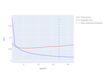
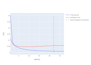
Both the training of \(M_1\) and the training of \(M_2\) are stopped restoring the epoch in which the model had the maximum f1-score
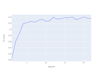
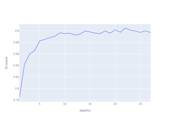
Note that the metric used to evaluate the performances of the model is not the accuracy since the number of possible roles (and also the number of possible predicates in \(M_2\)) is very high, and the given train dataset is imbalanced (there are roles that do not appear as a label in the training dataset)
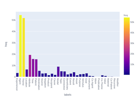
Moreover, since the tasks are multi-class problems, the adopted metric to evaluate the models is the f1-score.
These results are not the same as the ones obtained with a state-of-the-art model, but they are very close, so the proposed model is a good baseline to face the SRL task.