Introduction

In the last few decades, we have witnessed the great success of Deep Learning in many different tasks, due mainly to the usage of deep neural networks that have demonstrated incredibly generalization performances. However, in order to employ these tools in critical real-life task scenarios, we have to know the reason why a network has predicted a specific result, and considering the trend in designing deeper models to enhance their generalization capability, this reasoning process becomes hard to perform.

Nevertheless, Explainability comes to our rescue. Explainability is the research area of Artificial Intelligence whose goal is to reason the behaviour of neural networks given their black-box nature. Indeed, the prediction of a deep neural network is the result of many linear combinations with usually thousands of learnable parameters, followed by a non-linear activation. Therefore, there is no possibility to follow the exact map from the input to the prediction that the network performs. For this reason, ad-hoc methods need to be designed in order to clarify the decision-making process of such networks.

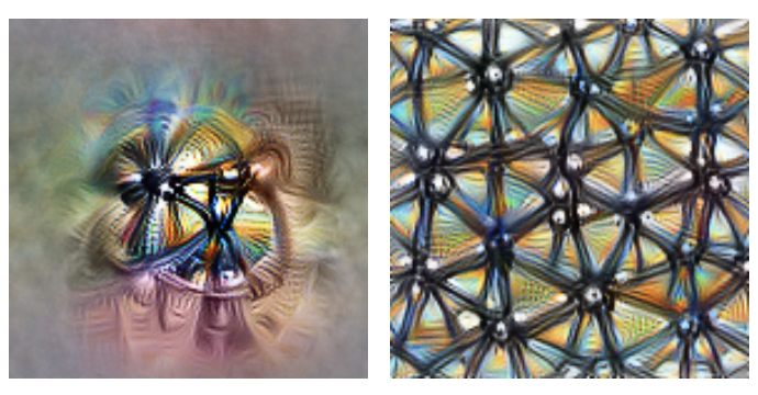
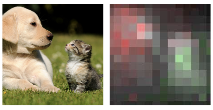
Two main directions are carried out in the Explainability field, namely Feature Visualization and Feature Attribution. In the former, once we have chosen a particular neuron (or a group of neurons) of a deep network, the task consists in generating the example that highly activates the selected neuron. While in the latter, the goal is to identify the relevant input features that cause a particular prediction for the network.

Feature Visualization via Input Optimization

A technique to perform Feature Visualization is called Input Optimization. The idea of such a technique is that: since we know that deep neural networks are differentiable with respect to their input, we can use the derivatives to iteratively tweak the input to make it cause a chosen behaviour of the network. Thus, starting from an input consisting of random noise and using the gradient information, we change the input to increase the activation of a previously selected neuron.

As suggested by the name, this technique is mathematically formulated as an optimization problem. In particular:

• given a model \(M\) with fixed weights \(\Theta\), and
• chosen a neuron (or a group of neuron) whose activation is indicated by the function \(h(\cdot)\)
• we look for the input \(\mathbf{X}\) that highly maximizes the activation \(h\)

Adversarial examples

Unfortunately, the optimization without any constraint results in a senseless example that highly excites the neuron anyway. These examples can be thought of as adversarial examples. Those might be useful to test the robustness of the neural network, but in order to figure out the representations learned by a neural network, they are useless. Thus, we need to inject some natural structure in the example we are synthesizing, and this can be obtained in three different ways: either we can train a prior and harness it during the optimization, or we can use some regularizer in the formula we are optimizing for, or we can impose some constraints the example may take during the optimization. In this work, we use a learned prior in order to obtain good visualizations.

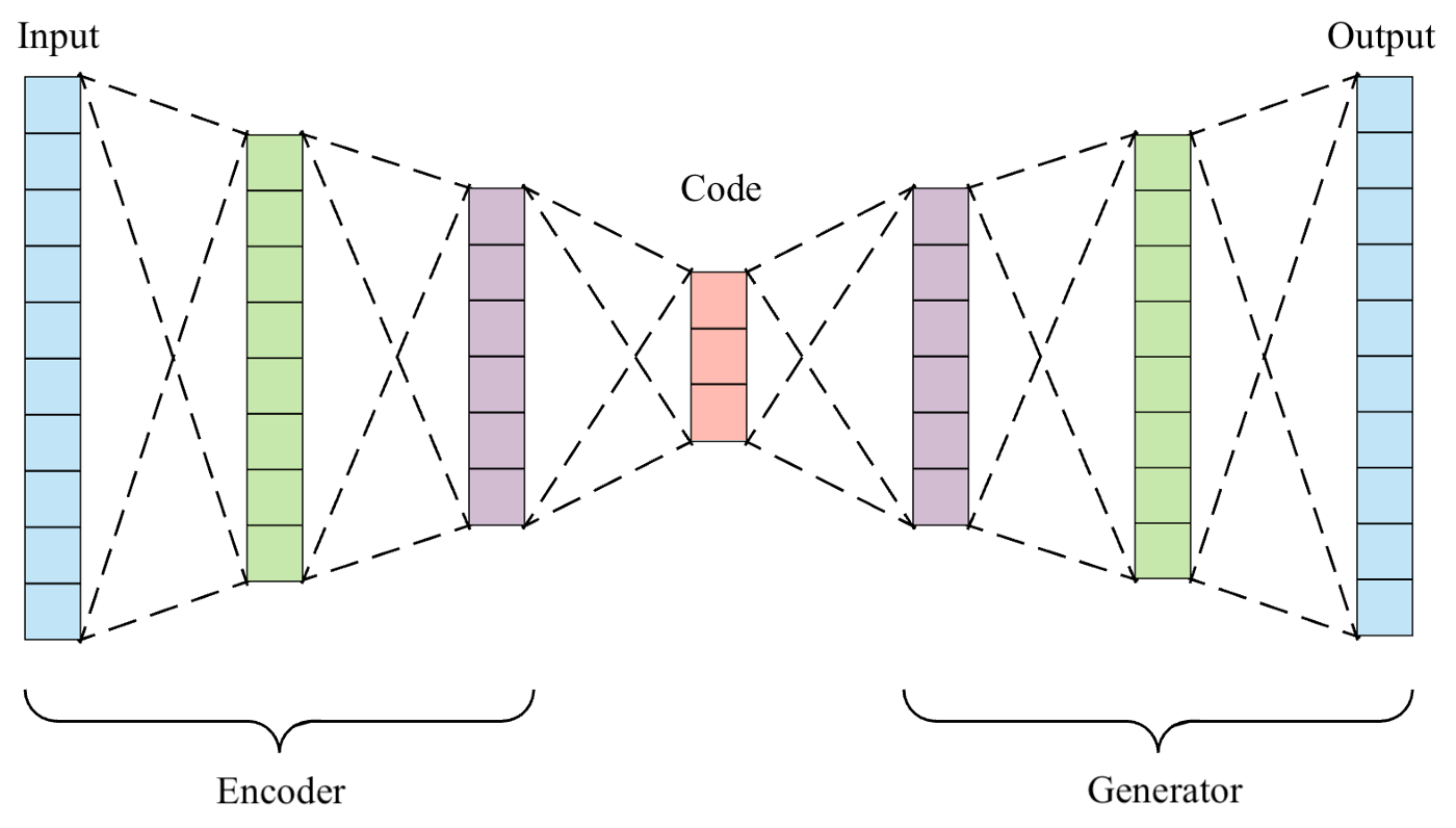
The idea of prior consists of the learning of a model of the real data distribution and then using it during the optimization to try to enforce that. In this work, the prior is a generative model that from a low-dimensionality representation, it returns an example of the real data. In this regard, the prior is trained using an autoencoder framework where just the generator represents the prior, thus only the generator is used during the optimization.

Feature Visualization on non-Euclidean data

Overall, Feature Visualization has led to remarkable insights for neural networks dealing with Euclidean data, in particular with images. Nonetheless, considering the increasing rise of the adoption of neural networks dealing with non-Euclidean data, so data like graphs or meshes where also the input structure is relevant, in this work, we use the Feature Visualization approach to provide explanations of these deep neural networks. Specifically, we deal with 3D point clouds, namely unordered sets of points that are easy-to-acquire, and for this reason, they are implemented in many deep learning tasks, like to represent the surrounded context of an autonomous car.

PointNet Classifier

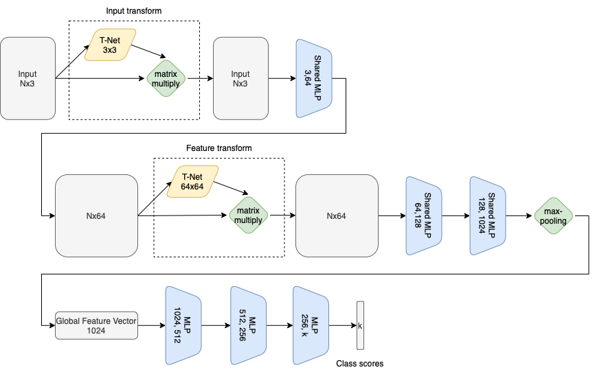
The network we are going to explain is the PointNet classifier (CR. Qi et al., 2017). In the figure, we can see the simple architecture of such a model. Namely, it is composed of multiple shared fully-connected layers between all the points that compose the input point cloud, followed by a max-pooling operation succeeded by several fully-connected layers. This structure gives the model some relevant properties, like permutation invariance and transformation invariance. In particular, given a point cloud of \(n\) points, this is represented by all the \(n!\) permutations of the points, thus all the permutations need to have the same prediction by the net. To obtain this, the authors use a symmetric function represented by the max-pooling operation that captures an aggregation of the n input points. Moreover, if a rigid transformation is applied to the point cloud the prediction of the network doesn’t have to change. Therefore, to obtain transformation invariance the authors of PointNet have used a little neural network called T-Net that predicts an affine transformation that at a first stage is applied to the input, and then, at a second stage, to the features extracted by an intermediate layer.

Training of the prior

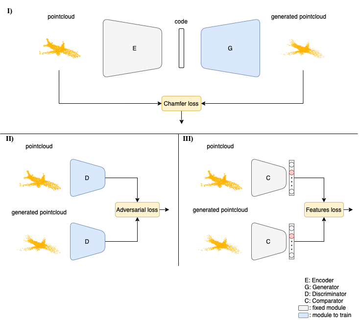
Instead, to train the prior we used a modified autoencoder network called, Adversarial AutoEncoder (A. Dosovitskiy et al., 2016). This framework is composed of four different networks: a fixed encoder \(E: \mathbb{R}^{N \times 3} \rightarrow \mathbb{R}^{\ell}\) that encodes a given point cloud in a latent space trying to preserve the relevant features of the input point cloud (it is represented by the PointNet classifier truncated at the Global Feature vector); a learnable generator \(G_{\theta}: \mathbb{R}^{\ell} \rightarrow \mathbb{R}^{N \times 3}\) that reconstructs a dataset example from a latent code (its architecture is represented in the following figure); a fixed comparator \(C: \mathbb{R}^{N \times 3} \rightarrow \mathbb{R}^{k}\) that extracts feature vectors from an input point cloud (it is represented by the whole PointNet classifier); and finally, a learnable discriminator \(D_{\phi}: \mathbb{R}^{N \times 3} \rightarrow \mathbb{R}\) which aims at distinguishing the original and generated point clouds (its architecture is represented in the following figure).

3D Adversarial AutoEncoder

Our 3D Adversarial AutoEncoder training, as can be seen from the figure, involves three steps that are performed simultaneously. Firstly, the encoder extracts a latent code from an input point cloud, and the generator reconstructs the original point cloud from the latent code. The similarity between the generated and original point cloud is measured by the chamfer loss. In the second step, the discriminator is fed with the original and generated point clouds, and the adversarial loss returns the confidence scores of the discriminator for each point cloud. Finally, the two-point clouds are given as input to the comparator that extracts the corresponding feature vectors. Those are then compared using a feature loss.

Losses

First of all, the Chamfer loss represents the reconstruction loss of the autoencoder. Let

• \(\mathbf{x}\) a point cloud from the dataset \(\mathbf{X}\),
• \(\mathbf{z}=E(\mathbf{x})\) the latent code obtained from \(\mathbf{x}\), and
• \(\tilde{\mathbf{x}}=G_{\theta}(\mathbf{z})\) the generated point cloud the Chamfer loss measures the distance between each point in the original point cloud \(\mathbf{x}\) to its nearest neighbour in the generated one \(\tilde{\mathbf{x}}\) and viceversa

Second, the feature loss measures the proximity between the feature vectors extracted by the comparator network. In fact, the distance is computed with the Mean Squared Error between the features vector of the original point cloud and the features vector of the generated point cloud.

Finally, the adversarial loss is introduced according to the Wasserstein GAN (I. Gulrajani et al., 2017) approach. Therefore, the training procedure is performed by alternating updates of generator parameters and the discriminator parameters. The generator is updated following the loss obtained by the sum of the chamfer loss and the feature loss minus the score returned by the discriminator on the generated point cloud

Note that, the minus sign is owing to the fact that the generator is trying to fool the discriminator, and thus it wants the discriminator to give a higher score for the generated point cloud.

By contrast, the discriminator parameters are updated according to this other loss

where the score of the discriminator on the generated point cloud is minimized, the scores on the original point cloud are maximized and additionally, the authors add a gradient penalty term to force the discriminator to approximate a \(1\)-Lipschitz function.

Input optimization procedure

Now, having the trained model to explain, namely the PointNet classifier, and the learned prior, namely the generator of the 3D-AAE, we can continue with the input optimization procedure. For this work, we selected the neuron to activate from the final layer of the PointNet classifier, specifically the class logits layer, thus we expect as output something specific to the class we have selected. To leverage the prior, the input to optimize lies in the latent space of the generator, and since we are going to maximize the activation of a neuron, the updates of the input are performed by making steps in the direction of the steepest ascent, namely the direction indicated by the gradients of the activation with respect to the input.

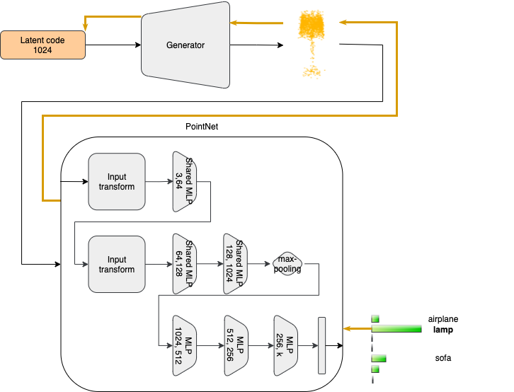
An overview of the pipeline of the input optimization process is shown in the previous figure. Starting from the latent code, we extract the point cloud using the generator that is then classified by the PointNet model obtaining a score for each of the considered classes. The orange bold arrow indicates the flow of the gradients that from the selected neuron of the last layer of PointNet goes through the point cloud in input back to the latent code of the Generator, which is then properly updated according to the activation we have obtained. More practically, the latent code is updated in such a way that the point cloud produced by the Generator, increasingly improves the activation of the selected neuron of PointNet responsible for the recognition of a particular class.

Results

To train and evaluate both the PointNet classifier and the 3D-Adversarial AutoEncoder architecture we use the ModelNet40 dataset. The dataset is composed of ~\(12\) thousand 3D shapes representing general objects. Out of those, \(9.843\) shapes build up the training dataset and \(2.468\) shapes build up the test dataset. Since our models deal with point clouds, the shapes are pre-processed. In particular, \(2.048\) points are uniformly sampled from the surface of each shape and then each obtained point cloud is centred and normalized into a unit sphere.

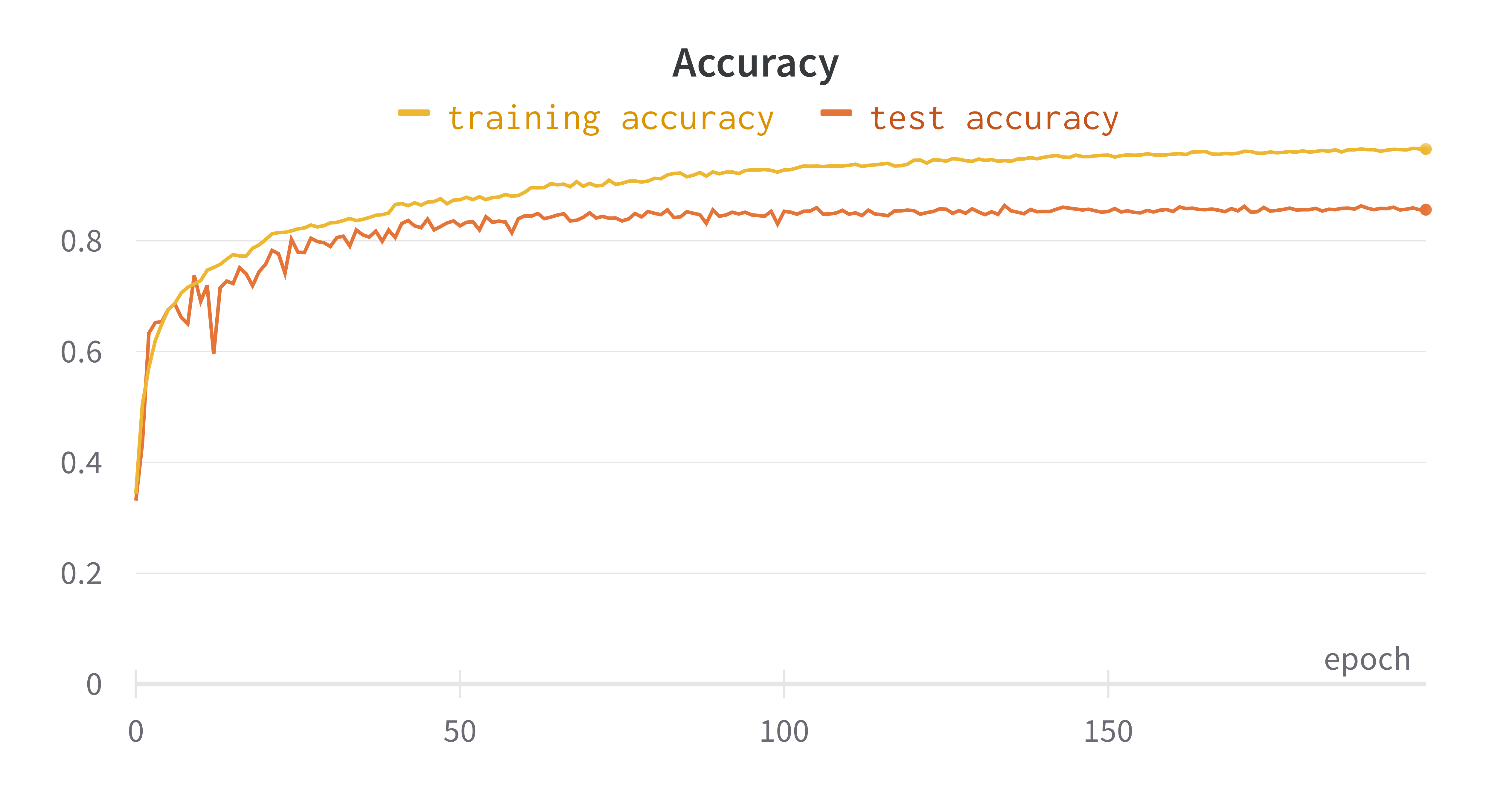
Since no checkpoint was provided by the authors of PointNet, we train the classifier from scratch, achieving an accuracy of ~\(86\)% that is almost the same performance as the original model.

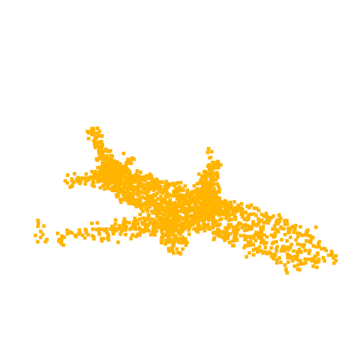
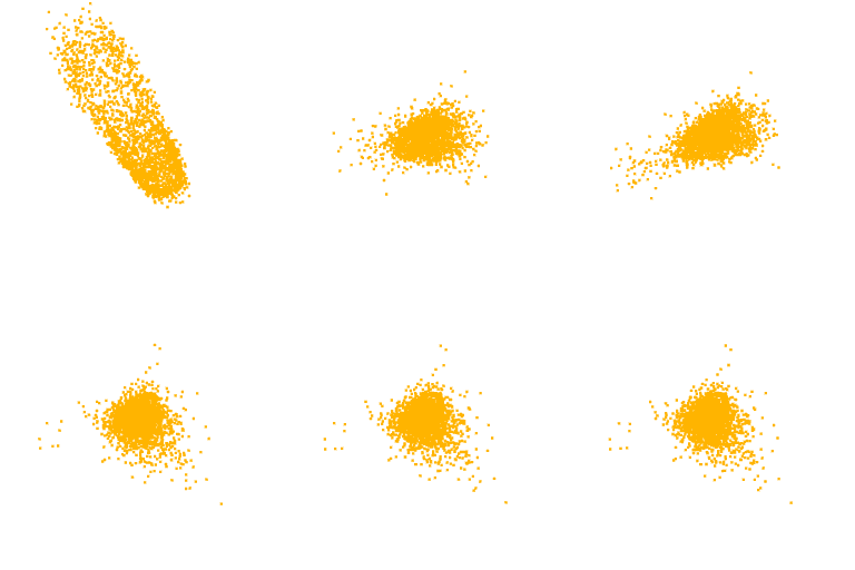
Instead, to evaluate the prior, we look at the reconstruction ability that the generator has on examples it has never seen during the training. in particular, we extracted from the test dataset of ModelNet40 one point cloud for each class and we evaluate how it is reconstructed by the generator as the training of the 3D-AAE goes on. We can see from the figures that the reconstructed point clouds approach the original one, so we can state that the generator has learned to represent a point cloud from a latent code.

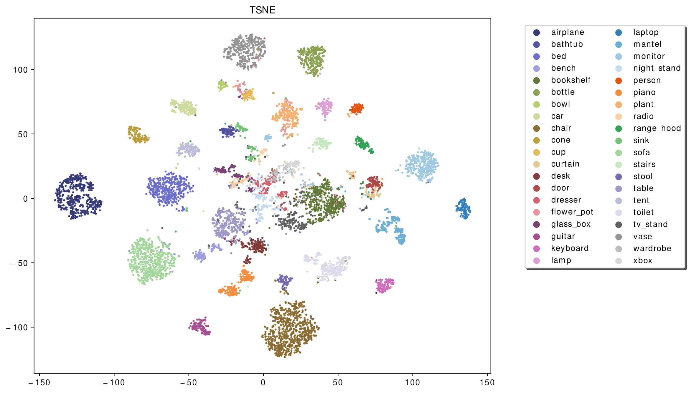
To better support this statement, we also look at the latent space, where we can see that the classes are clustered in a meaningful way, namely latent codes representing the features of the same class are close together. Thus, we expect that by sampling a code near to the cluster of a class and then giving it as input to the Generator, we obtain a point cloud according to that class. The latent space represents also the space in which we restrict our search during the optimization process.

Input Optimization results

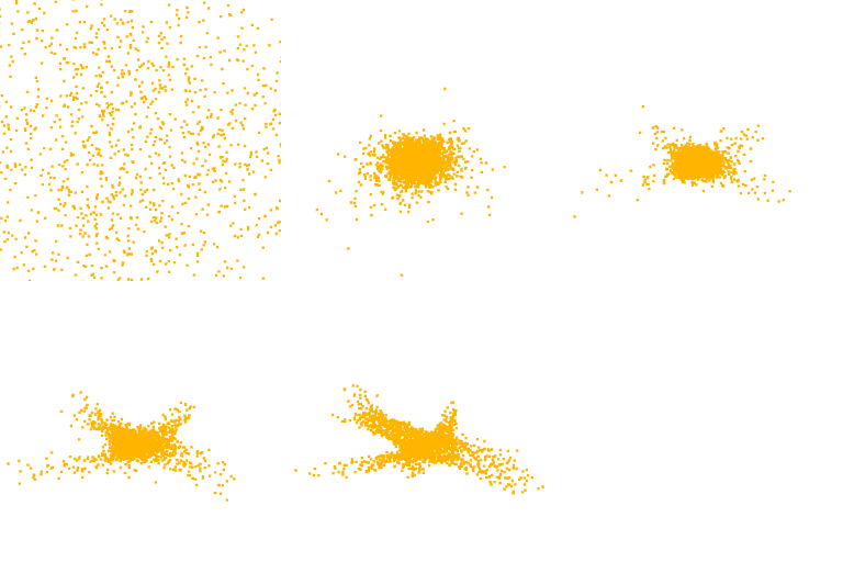
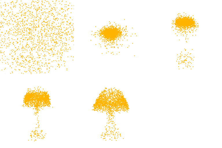
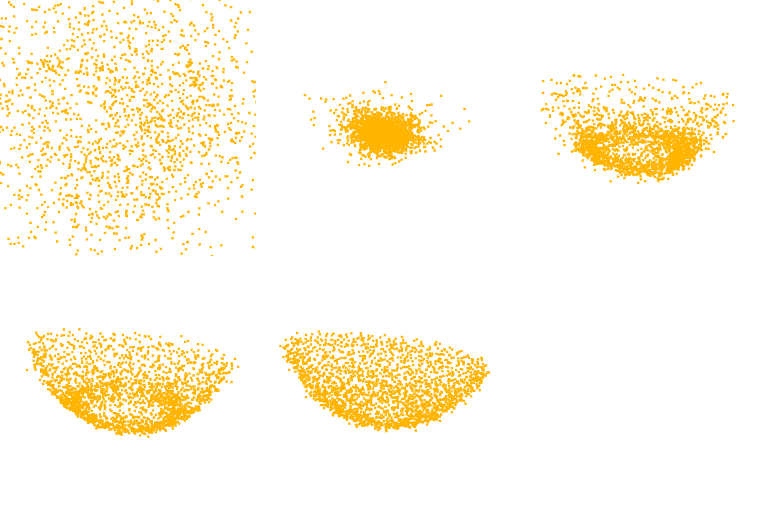
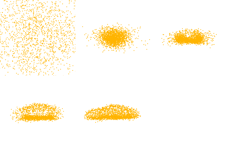
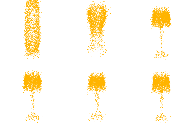
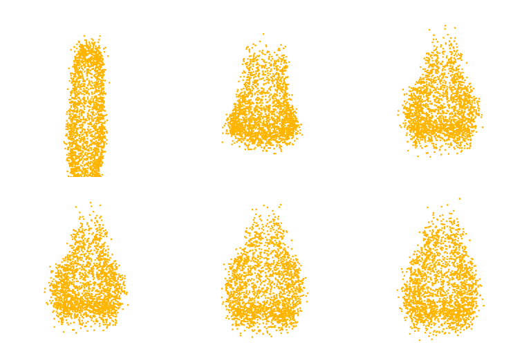
As previously mentioned, for the optimization we selected the neuron from the class logits layer, thus in output we expect to visualize the part of the point cloud on which the neuron focuses. In fact, as can be seen from the optimizations of the classes Lamp, Vase and Stool, we obtain point clouds reliable compared with the class for which the neuron we are optimizing for is responsible.

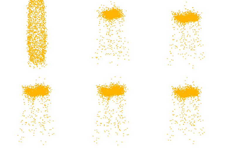
Unfortunately, one of the limitations of this approach is that not all the visualizations produced are interpretable. In fact, as can be seen from the optimization for the class airplane, what we obtain is something that possibly resembles an airplane (as can be inferred by the two wings we obtain at the end of the optimization), but is not clear as the previous classes. This behaviour is due to the fact that, in general, a neuron can be activated in different directions, and each direction can lead to different parts of the point cloud. To overcome this problem, all the possible directions needs to be investigated but given the high number of neurons that compose a network and considering the infinite directions, it is a hard task to perform as well as time-consuming.

Conclusions

To sum up, in this work we have exhibited an explanation approach working with neural networks dealing with 3D data, in particular with 3D point clouds. Moreover, To make the approach work in this context, we have also proposed a new way to learn a prior leveraging a generative framework named 3D Adversarial AutoEncoder in order to inject some prior for the structure of the synthesised point cloud.

Finally, since Explainability of models dealing with non-Euclidean data is still a poorly investigated field, this work can be considered as a starting point for ongoing research in this direction, and for this reason, it can be extended in several ways:

• excite different neurons in the middle layers of the models to have more insights into the hidden features the network has learned, but we have also to come out with a reasonable way to represent high-dimensionality data in a 3D space.
• design novel approaches to learn a prior that is as general as possible and that can be used equally to diverse architectures without the need to train it from scratch every time.